Example: Lorenz63 Equations
Problem Description
As a first tutorial we will use the famous equations Lorenz equations. The governing ODEs are:
where \(\sigma, R, b\) are physical parameters, the dot denotes the differentiation with respect to the time \(t\), respectively.
Inputing the Lorenz Model
To use cnspy generate the cns code, you need to tell cnspy what the functions will be calculate.
Firstly, we importing all necessary packages:
[ ]:
import sympy as sp
import time
from cnspy import cns
from cnspy import method
from cnspy import adaptive, adaptive_parameters
import mpmath
mpmath.mp.dps =500
Then, we create the Lorenz equations through Sympy:
[ ]:
t = sp.symbols(r't')
sigma,R,B = sp.symbols(r'\sigma, R, B')
u=sp.symarray('x', 3)
f1=sigma*(u[1]-u[0])
f2=R*u[0]-u[1]-u[0]*u[2]
f3=u[0]*u[1]-B*u[2]
fun=[f1,f2,f3]
Generate CNS C code of Lorenz equations
To generate the CNS code, just simply use the cns function, and the simulation is set up with several parameters and configurations as detailed below:
lorenz63: This is the variable where the simulation object is stored.cns(funcs=fun, name="lorenz63", ...): Thecnsfunction is called to initialize the simulation. Thefuncs=funargument specifies the function(s) used for the system of equations. The name of the simulation is set to"lorenz63".method=method('TS'): The method used for solving the equations is specified as'TS'(likely referring to a time-stepping method or a particular solver).inits=[[u[0],"-15.8"], [u[1],"-17.48"], [u[2],"35.64"]]: This defines the initial conditions for the system. The three initial values correspond to the state variables of the Lorenz system, presumably representing the initial values for the three variables (u[0],u[1],u[2]) at timet=0.paras=[[sigma,"10"], [R,"28"], [B,"8/3"]]**: This defines the parameters of the Lorenz-63 system.tspan=(0,1000): The simulation will run from timet=0tot=1000.saveat=0.1: Data will be saved at intervals of 0.1 units of time.lyap=0.91: A parameter related to the Lyapunov exponent, which measures the rate of separation of trajectories in chaotic systems.adaptive=adaptive('t','order','wordsize',delta_T=50,remaining_T=300,gamma=1.1): This sets the adaptive control for the simulation, specifying:delta_T = 50: The changing interval of the number of significant digits and order.remaining_T = 300: The remaining time for the stabilization.gamma = 1.1: The safety factor larger than 1.
mpi=True: This indicates that the simulation will be parallelized using MPI (Message Passing Interface), enabling the use of multiple processors.run_os='posix': Specifies the operating system to run the simulation, in this case, POSIX-compliant systems (e.g., Linux or macOS).printprecision=500: The precision of the printed output is set to 500 decimal places.numofprocessor=64: The simulation is configured to use 64 processors for parallel computation.
[ ]:
lorenz63=cns(funcs=fun,name="lorenz63",\
           method=method('TS'),\
           inits=[[u[0],"-15.8"],[u[1],"-17.48"],[u[2],"35.64"]],\
           paras=[[sigma,"10"],[R,"28"],[B,"8/3"]],\
           tspan=(0,1000),\
           saveat=0.1,\
           lyap=0.91,\
           adaptive=adaptive('t','order','wordsize',delta_T=50,remaining_T=300,gamma=1.1),\
           mpi=True,\
           run_os= 'posix',\
           printprecision= 500,\
           numofprocessor=64)
Note
The word size of the input is in binary digits, and the word size 3072 will be 924 in decimal digits. The conversion formula is: :math:P_{dec} = P_{bin}\cdot \lg 2. It is worth mentioning that the double accuracy is 15 decimal places ( :math:52\cdot\lg 2=15).
Finally, the code will be generated by calling the generate_c_code():
[ ]:
lorenz63.generate_c_code()
Run the job on a cluster
Then, we can run the code on a cluster with 64 processors. You can use the following code to do that:
[ ]:
from cnspy import cluster
SL = cluster.slurm_script(node='cu10', qos='super', np=lorenz63.numofprocessor, jobname = lorenz63.name)
HN = cluster.ssh(config_path = '<path_to_your_config_file>')
lorenz63.run(HN,SL)
And ofcourse, you can run the code on your local machine:
cd lorenz63/ccode/
make
mpirun -n 4 lorenz63
Finally, we can read the data and generate a RK4 solution to compare:
[ ]:
#read result
lorenz63.read_cnssol()
#rk4 result
lorenz63.quick_run()
Similarly, we can run the Lorenz96 model only adaptive in time to generate a examine CNS case with higher order and number of significant digits:
[ ]:
lorenz63_higher=cns(funcs=fun,name="lorenz63_higher",\
           method=method('TS',order=800,nosd=500),\
           inits=[[u[0],"-15.8"],[u[1],"-17.48"],[u[2],"35.64"]],\
           paras=[[sigma,"10"],[R,"28"],[B,"8/3"]],\
           tspan=(0,1000),\
           saveat=0.1,\
           lyap=0.91,\
           adaptive=adaptive('t'),\
           mpi=True,\
           printprecision= 500,\
           numofprocessor=64)
[ ]:
lorenz63_higher.generate_c_code()
[ ]:
from cnspy import cluster
SL = cluster.slurm_script(node='cu5', qos='super', np=lorenz63_higher.numofprocessor, jobname = lorenz63_higher.name)
HN = cluster.ssh()
lorenz63_higher.run(HN,SL)
[ ]:
#read result
lorenz63_higher.read_cnssol()
#rk4 result
lorenz63_higher.quick_run()
Then, to compare the adaptive in order and wordsize, we can use the following code:
[ ]:
lorenz63_fix=cns(funcs=fun,name="lorenz63_fix",\
           method=method('TS',order=617,nosd=411),\
           inits=[[u[0],"-15.8"],[u[1],"-17.48"],[u[2],"35.64"]],\
           paras=[[sigma,"10"],[R,"28"],[B,"8/3"]],\
           tspan=(0,1000),\
           saveat=0.1,\
           lyap=0.91,\
           adaptive=adaptive('t'),\
           mpi=True,\
           printprecision= 500,\
           numofprocessor=64)
[ ]:
lorenz63_fix.generate_c_code()
[ ]:
from cnspy import cluster
SL = cluster.slurm_script(node='cu10', qos='super', np=lorenz63_fix.numofprocessor, jobname = lorenz63_fix.name)
HN = cluster.ssh()
lorenz63_fix.run(HN,SL)
[ ]:
#read result
lorenz63_fix.read_cnssol()
#rk4 result
lorenz63_fix.quick_run()
Plot the results
Now, it’s time to compare and plot the results.
Firstly, we define the relative error function by:
where \(N_d\) is the number of the variable~(i.e. dimensions of the model), \(x_i^{'}(t)\) and \(x_i(t)\) are two CNS results with different level of the background numerical noise, respectively.
The code can be defined by:
[ ]:
import sympy as sp
def relative_error(y1, y2):
    for j in range(len(y1[:,0])):
        if j == 0:
            era = [sp.Float(abs(y1[j,i] - y2[j,i])) for i in range(len(y1[0,:]))]
            erb = [sp.Float(abs(y2[j,i])) for i in range(len(y1[0,:]))]
        else:
            era = [ era[i] + sp.Float(abs(y1[j,i] - y2[j,i])) for i in range(len(y1[0,:]))]
            erb = [ erb[i] + sp.Float(abs(y2[j,i])) for i in range(len(y1[0,:]))]
    return [era[i] / erb[i] for i in range(len(era))]
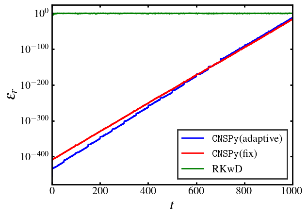
Then, we can plot the relative error of the three method via the examine case:
[ ]:
import matplotlib.pyplot as plt
from matplotlib import rc
rc("legend",fancybox=False)
rc('text', usetex=True)
rc('text.latex', preamble=r'\usepackage{amsmath} \boldmath')
rc('patch',linewidth=2)
font = {'family' : 'serif',
        'serif':['Times'],
        'weight' : 'bold',
        'size'   : 16}
rc('font', **font)
from matplotlib.ticker import FuncFormatter

x = lorenz63.cnssol.t
y1 = relative_error(lorenz63.cnssol.y, lorenz63_higher.cnssol.y)
y2 = relative_error(lorenz63_fix.cnssol.y, lorenz63_higher.cnssol.y)
y3 = relative_error(lorenz63.qrsol.y, lorenz63_higher.cnssol.y)
def log_formatter(x, pos):
    return "$10^{{{:d}}}$".format(int(x))

formatter = FuncFormatter(log_formatter)

fig, ax = plt.subplots()

y11 = list(map(lambda x:sp.log(x, 10), y1))
y22 = list(map(lambda x:sp.log(x, 10), y2))
y33 = list(map(lambda x:sp.log(x, 10), y3))
ax.plot(x, y11,label=r'\texttt{CNSPy}(adaptive)',linestyle="-",linewidth=2,color="blue")
ax.plot(x, y22,label=r'\texttt{CNSPy}(fix)',linestyle="-",linewidth=2,color="red")
ax.plot(x, y33,label=r'RKwD',linestyle="-",linewidth=2,color="green")
ax.yaxis.set_major_formatter(formatter)
ax.set_xlim(0,1000)
ax.set_xlabel(r'$\boldsymbol{t}$', fontsize=22, fontweight='bold')
ax.set_ylabel(r'$\boldsymbol{\epsilon_r}$', fontsize=22, fontweight='bold')
ax.tick_params(direction="in",top=True,right=True,width=2)
ax.legend(edgecolor="inherit",loc="best")
for location in  ["left", "right", "top", "bottom"]:
    ax.spines[location].set_linewidth(2)

fig.savefig("lorenz63_error.eps",bbox_inches='tight')
The PostScript backend does not support transparency; partially transparent artists will be rendered opaque.
Failed to find a Ghostscript installation.  Distillation step skipped.
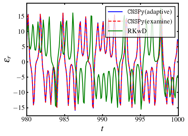
We can also check the last 20 unit time of the simulation:
[ ]:
#plot phase space
import matplotlib.pyplot as plt
from matplotlib import rc
rc("legend",fancybox=False)
rc('text', usetex=True)
rc('text.latex', preamble=r'\usepackage{amsmath} \boldmath')
rc('patch',linewidth=2)
font = {'family' : 'serif',
        'serif':['Times'],
        'weight' : 'bold',
        'size'   : 16}
rc('font', **font)
fig, ax = plt.subplots()
ax.plot(lorenz63.cnssol.t[9800:10000],lorenz63.cnssol.y[0,9800:10000],label=r'\texttt{CNSPy}(adaptive)',linestyle="-",linewidth=2,color="blue")
ax.plot(lorenz63_higher.cnssol.t[9800:10000],lorenz63_higher.cnssol.y[0,9800:10000],label=r'\texttt{CNSPy}(examine)',linestyle="--",linewidth=2,color="red")
ax.plot(lorenz63.qrsol.t[9800:10000],lorenz63.qrsol.y[0,9800:10000],label=r'RKwD',linestyle="-",linewidth=2,color="green")

ax.set_xlim(980,1000)
ax.set_xlabel(r'$\boldsymbol{t}$', fontsize=22, fontweight='bold')
ax.set_ylabel(r'$\boldsymbol{\epsilon_r}$', fontsize=22, fontweight='bold')
ax.tick_params(direction="in",top=True,right=True,width=2)
ax.legend(edgecolor="inherit",loc="best")
for location in  ["left", "right", "top", "bottom"]:
    ax.spines[location].set_linewidth(2)

fig.savefig("lorenz63_x1.eps",bbox_inches='tight')
The PostScript backend does not support transparency; partially transparent artists will be rendered opaque.
Failed to find a Ghostscript installation.  Distillation step skipped.
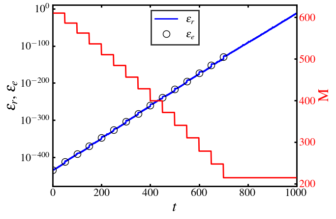
Or check the adaptive process of the order and error in the whole calculated time:
[ ]:
import numpy as np
import mpmath
def order_nosd_time(system):
    magic_number = system.adptv_para.magic_number
    gamma = system.adptv_para.gamma
    remaining_T = system.adptv_para.remaining_T
    lyap = system.lyap
    tmax = system.tspan[1]
    time = [i for i in range(0, tmax+1)]
    delta_T = system.adptv_para.delta_T
    order = np.zeros(len(time))
    nosd = np.zeros(len(time))
    desire_error = []
    desire_time = []
    for i in range(0, len(time)):
        if i % delta_T == 0 and i <= tmax - remaining_T:
            nosd[i] = int(gamma*lyap*(tmax-i)/np.log(10.0))
            desire_error.append(10**(-mpmath.mp.mpf(nosd[i])))
            desire_time.append(i)
        else:
            nosd[i] = nosd[i-1]
        order[i] = int(magic_number[0]*nosd[i]*nosd[i]+magic_number[1]*nosd[i]+magic_number[2])
        order[-1] = order[-2]
        nosd[-1] = nosd[-2]

    return time, np.array(desire_time), order, nosd, np.array(desire_error)

import matplotlib.pyplot as plt
from matplotlib import rc
rc("legend",fancybox=False)
rc('text', usetex=True)
rc('text.latex', preamble=r'\usepackage{amsmath} \boldmath')
rc('patch',linewidth=2)
font = {'family' : 'serif',
        'serif':['Times'],
        'weight' : 'bold',
        'size'   : 16}
rc('font', **font)
from matplotlib.ticker import FuncFormatter

x = lorenz63.cnssol.t
y1 = relative_error(lorenz63.cnssol.y, lorenz63_higher.cnssol.y)
t_lorenz63, desire_time_lorenz63, order_lorenz63, nosd_lorenz63, desire_error_lorenz63 = order_nosd_time(lorenz63)
def log_formatter(x, pos):
    return "$10^{{{:d}}}$".format(int(x))

formatter = FuncFormatter(log_formatter)

fig, ax1 = plt.subplots()
ax2 = ax1.twinx()
y11 = list(map(lambda x:sp.log(x, 10), y1))
y22 = list(map(lambda desire_time_lorenz63:sp.log(desire_time_lorenz63, 10), desire_error_lorenz63))
ax1.plot(x, y11,label=r'$\boldsymbol{\epsilon_{r}}$',linestyle="-",linewidth=2,color='blue')
ax1.plot(desire_time_lorenz63, y22,label=r'$\boldsymbol{\epsilon_{e}}$',marker="o", markersize=10,color='none', markerfacecolor='none', markeredgecolor="black")
ax2.plot(x[::10], order_lorenz63,label='order',linestyle="-",linewidth=2,color='red')
ax2.tick_params(direction="in",axis='y', labelcolor='red',width=2)
ax2.set_ylabel(r'M', fontsize=22, color='red', fontweight='bold')
ax1.yaxis.set_major_formatter(formatter)
ax1.set_xlim(0,1000)
ax1.set_xlabel(r'$\boldsymbol{t}$', fontsize=22, fontweight='bold')
ax1.set_ylabel(r'$\boldsymbol{\epsilon_r}$, $\boldsymbol{\epsilon_e}$', fontsize=22, fontweight='bold')
ax1.tick_params(direction="in",top=True,width=2)
ax1.legend(edgecolor="inherit",loc="upper center")
for location in  ["left", "right", "top", "bottom"]:
    ax1.spines[location].set_linewidth(2)

fig.savefig("algorithm_lorenz63.eps",bbox_inches='tight')
The PostScript backend does not support transparency; partially transparent artists will be rendered opaque.
Failed to find a Ghostscript installation.  Distillation step skipped.